The Impact of Portfolio Constraints
Summary: Very few fund managers really understand the impact of portfolio constraints on their ultimate results. While they spend a great deal of time and analytical effort on understanding their alpha ideas, comparatively little is spent on the inputs that define their portfolio’s shape. Building on the 3 Cs framework Sherpa uses to help managers define a robust portfolio problem definition, this piece discusses how the Candidate Portfolio Analysis tool can help PMs quantify the impact of different shape decisions. By better understanding this non-intuitive portfolio dynamic fund managers can make better decisions that improve their chances of achieving the portfolio outcome they desire.
Watch the related “Impact of Your Constraints” webinar at the link.
How much do your constraints matter in your portfolio? Do you even know?
In previous webinars and Insights posts we introduced the Sherpa 3 Cs (Complete, Coherent, Consistent) framework for evaluating a portfolio problem definition.
However, as we saw in the 3 Cs discussion, the portfolio manager actually has control over many of their stated constraints.
In this post we’ll introduce a quantitative framework using the Sherpa Candidate Portfolios Analysis to illustrate the impact of portfolio constraint decisions on portfolio outcomes.
By combining the 3 Cs framework with the Candidate Portfolio Analysis tool PMs gain a better understanding of what they are trying to achieve with their portfolio. As a result, they can ensure they are setting up the problem to have the best chance of achieving the outcome they desire.
Review: The Candidate Portfolios Analysis Tool
The Sherpa Candidate Portfolio Analysis constructs many eligible “candidate” portfolios using the same selections, objectives and constraints to show portfolios the PM COULD have constructed. For a more detailed refresher check out our Insights post here or our webinar on the topic here.
Candidate Portfolio Analysis helps PMs understand the range of potential outcomes and paths given their ideas and shape. Depending on the problem definition the range may be very tight (ie highly constrained) or may be very wide (ie loosely constrained).
In our prior posts we have largely discussed this in terms of understand the drivers of what made a portfolio “good” ex-post:
- Asset Selection
- Impact of Portfolio Construction
However, this tool can also help illustrate the impact of different portfolio shapes.
Analyzing the range of outcomes from different shapes created using the same ideas helps PMs better understand the impact of their portfolio constraints and make more informed portfolio construction decisions.
Additional Metrics to Understand the Candidate Portfolios
To better understand the output of the Candidate Portfolio analysis we can add a few additional metrics to describe the average and range of outcomes.
- The Median or Average Return helps illustrate the direction of the distribution and the alpha in the ideas
- Return Spreads (90 – 10 or 75 – 25) help illustrate the width of the range of possible outcomes given that set of ideas and portfolio shape – how much can you hurt or help with construction
- Traditional Risk and Return Statistics by Candidate Portfolio such as volatility, drawdown, etc describe the characteristics of any particular portfolio composition for easy comparison
There are of course many more complex ways to describe the outputs of the Candidate Portfolio Analysis, but we will leave that discussion for another session. We also won’t focus as much on risk characteristics in this discussion but will discuss that in a future post.
To Illustrate How This Works, Let’s Consider a Simple Example
To illustrate the impact of changing constraints on possible portfolio outcomes, let us consider two levers most Sherpa client PMs have significant discretion over – the Asset Max Sizes for the largest positions and the Level of Risk they want the portfolio to take.
These typically go hand in hand. Increasing the amount of freedom in portfolio construction by increasing the maximum asset weights facilitates taking an increasing level of risk. However, these are two distinct choices, so we will separate these into Low, Medium and High for each.
- Asset Max Sizes – Low, Medium, High
- Level of Risk – Low, Medium, High
To show how these problem definition decisions impact possible outcomes we will first consider 4 portfolios differing on these decision axes. This will begin to show us the impact of changing constraints on possible outcomes using the Candidate Portfolios Analysis.
- L-L – Low Level of Risk and Low Max Asset Size (our initial baseline)
- M-M – Medium Level of Risk and Medium Max Asset Size
- M-H – Medium Level of Risk and High Max Asset Size
- H-H – High Level of Risk and High Max Asset Size
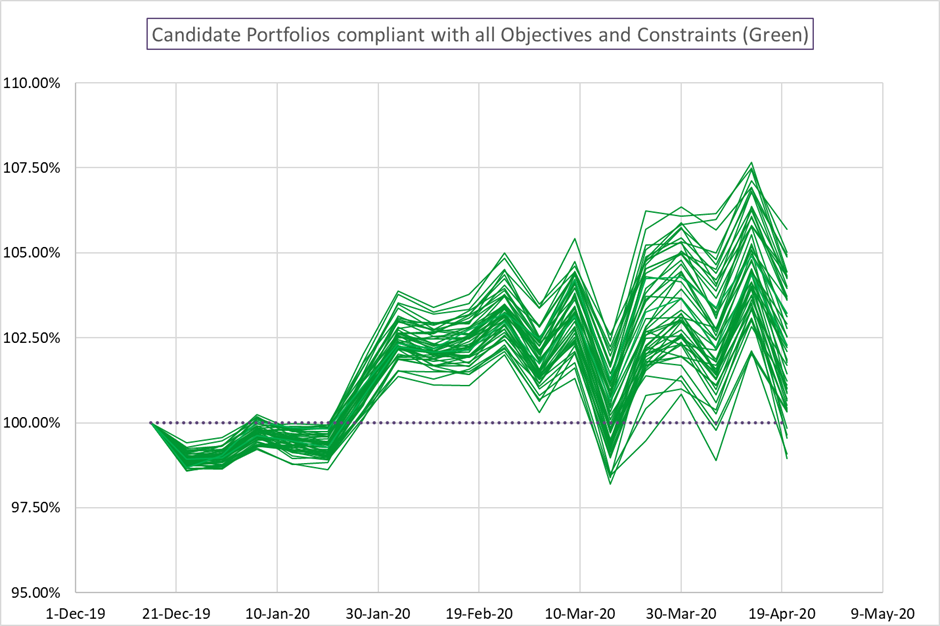
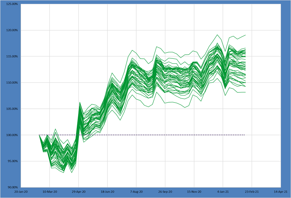
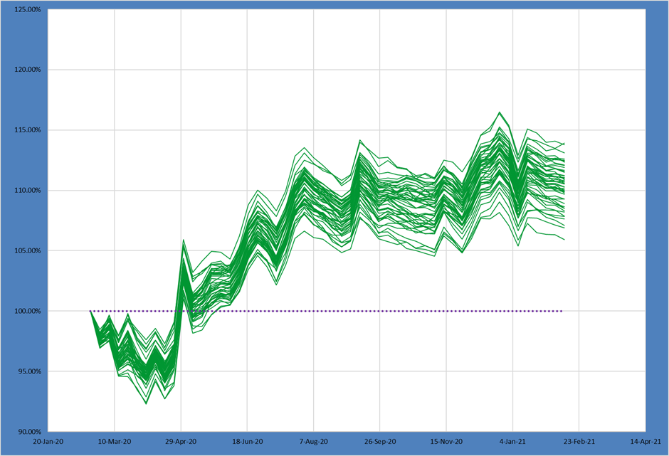
Low Risk and Low Max Asset Sizes – Our Starting Point

The Low Risk-Low Max portfolio is relatively more tightly constrained vs the other 3 portfolios. Lower asset max sizes mean less room for variation at the individual asset level and focusing on risk reduction means a tighter range of risk outcomes.
The 50th percentile outcome in this Candidate Portfolio Analysis produced a 13.24% return – not bad at all! Any all outcomes produced positive double-digit returns.
The spread of outcomes illustrates the potential impact of portfolio construction. The spread between the 75th and 25th percentiles was almost 2.5% over the period and the 90th – 10th spread was almost 5%!
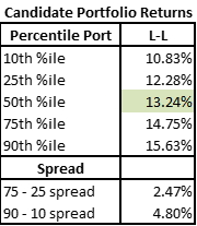
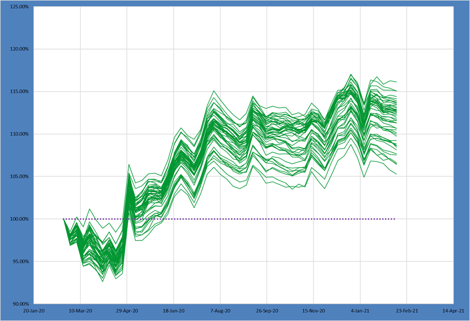
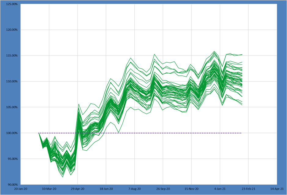
Medium Risk and Medium Max Sizes – Increases Variation + Returns
Now the next portfolio increases both the maximum asset size as well as the amount of acceptable portfolio risk. The portfolio is less tightly constrained than the Low-Low portfolio above.

Just as we would anticipate the range of possible outcomes is much wider. The spreads have increased substantially up to 4% on the 75th – 25th and over 6% on the 90th – 10th!
Further, we can see the 50th percentile portfolio produced 13.48% returns – higher than the median portfolio in the prior Low Risk – Low Max shape.

Loosening the portfolio constraints and increasing risk delivered potentially higher returns, but with much greater variation in outcomes.
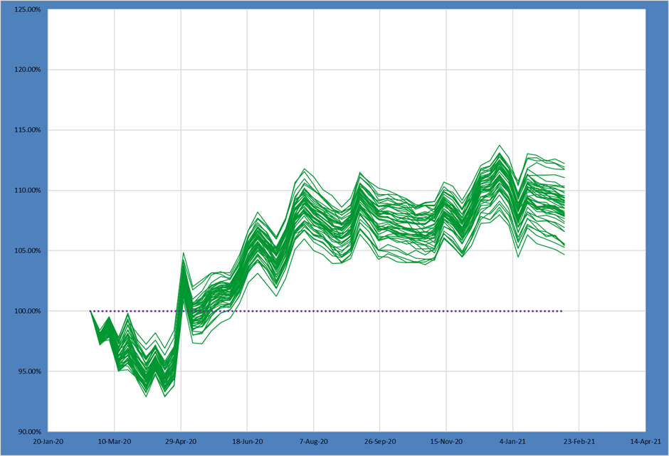
Medium Risk and High Max Sizes – Even Greater Variation + Returns
In the next example we further loosen the max asset size constraint while retaining the medium level of risk. This should give a set of portfolios that have greater variation than the Med-Med example above but without taking substantially greater risk.
As anticipated, the spread of outcomes has widened even further compared to the Med-Med portfolio.
At the same time, the 50th percentile return increased again as well! As returns have generally increased as we’ve allowed greater maximum asset weights and taken more risk, this would suggest the Low-Low portfolio we start with wasn’t taking enough risk given the alpha in the underlying ideas.

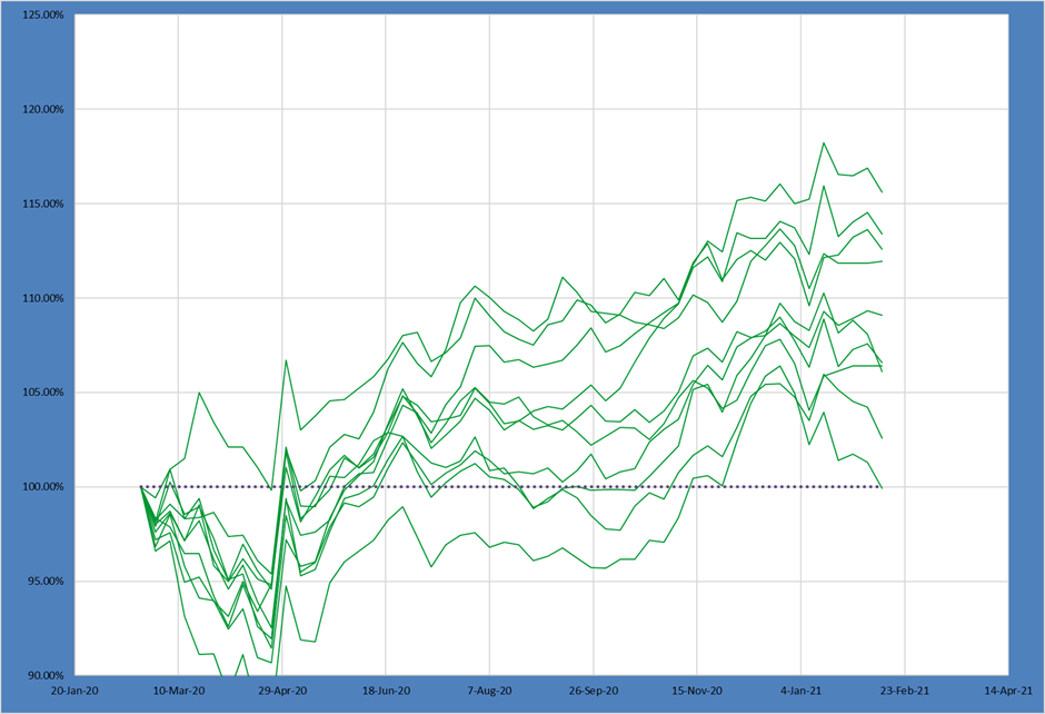
High Risk and High Max Sizes – Huge Outcome Variation, Return lower?
Let us look at what happens when we push that idea a step further – high max asset sizes and high risk.
While the spread of possible outcomes increases yet again, the average return begins to dip!

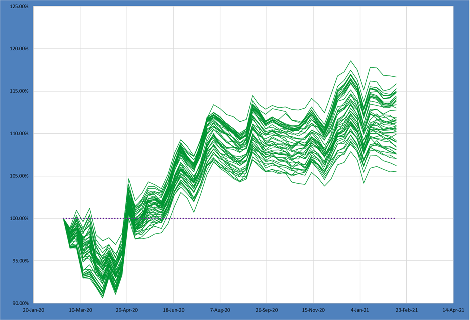
Comparing the Results, Spread Increased as More Freedom Allowed
Simple charts comparing the 4 portfolios above rather clearly illustrate how changing these two simple levels – maximum asset size and level of risk – impact the possible outcomes we could see with the ideas and other constraints held constant.
As we allow for greater size variation and take more risk, the spread of possible outcomes increases at both the 75th – 25th and 90th – 10th levels.
At the same time, the median Candidate Portfolio’s return increases somewhat as we go from L-L to M-M to M-H, before dropping sharply when we move to H-H.
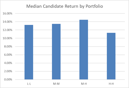
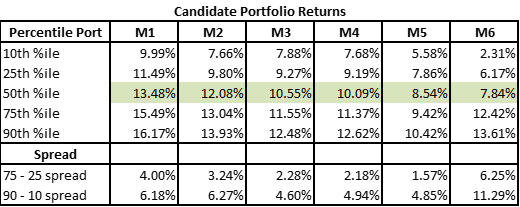
The full results are summarized below for reference.
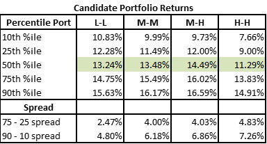
With positive alpha, moving from the Low Risk profile to the Medium Risk profile increased returns. Increasing the maximum asset weights further increased returns, albeit with a larger spread, as there was more freedom in portfolio construction.
However, expanding this to a High Risk profile with the higher level of freedom led to a dramatic drop in results. The portfolios were taking more risk than the alpha quality in the ideas!
There is an interaction between alpha quality and risk taking at both the portfolio level and the asset freedom level. If you take more risk than your alpha quality and allow too much freedom, your results can suffer.
This Method Illustrates the Impact of Constraints on Outcomes
Most often the PM drives the risk level and asset max portfolio shape decisions.
However, the other constraints that make up the portfolio shape can be just as impactful on potential portfolio outcomes – whether the PM can control them or not.
When the PM understands how Hard constraints imposed on them impact the portfolio they can have a more meaningful discussion with the relevant stakeholders of the objectives of that constraint.
For Soft constraints, this understanding gives the PM another potential tool to create a portfolio that best takes the risk they want it to take.
Let’s Look at the Impact of Various Constraint Changes
To see how different constraints impact potential portfolio outcomes, lets hold the risk level and asset maximum sizes constant and look at other types of constraints that may be placed on the portfolio.
To illustrate the concept, we will examine 6 examples below:
- M1 – Baseline Medium-Medium portfolio shape from previous section
- M2 – Same as M1 except all assets must be included at min of 50bps size (no small positions or assets excluded)
- M3 – Same as M1 except non-Asia region names must be at least 20% of portfolio (region constraint)
- M4 – Same as M3 but adding a constraint that sectors have max of 2% deviation from benchmark (sector constraint)
- M5 – Same as M4 but adding the asset inclusion constraint from M2 (all of the M2, M3 and M4 constraints)
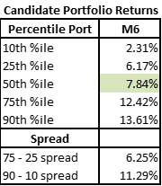
- M6 – Same as M3 but any position must be min of 3% above benchmark or not included (0% wt)
M1: ORS Baseline Medium Risk, Medium Asset Max Portfolio Above
This first example serves as our baseline – a relatively unconstrained portfolio construction except basic asset max and risk specifications.
As discussed before, this set of ideas clearly has meaningful alpha but with relatively few constraints it might be expressed in many different actual portfolio paths.

M2: M1 with All Asset Constraint
For the first constraint, we simply specify that the portfolio must included all assets on the PM’s list and each asset weight must be a minimum of 50 basis points.
The Candidate Portfolio Analysis again helps us visualize the impact of this constraint change on the set of possible portfolio outcomes relative to our baseline M1.
Adding this constraint moves our distribution down – the 10th, 50th and 90th percentile outcomes are all lower return than the comparable percentiles in portfolio M1.

This makes intuitive sense as the more constrained portfolio is not “free” to express the alpha in an unconstrained manner.
Interestingly while the 75th – 25th spread narrows somewhat, the 90th – 10th spread is slightly larger.
M3: M1 with Region Constraint
Now let us instead add a constraint on the region positioning of the portfolio. Again we would anticipate that adding this constraint changes the possible outcomes and the Candidate Portfolio Analysis gives us a lens to quantify the magnitude of the change.
The region constraint produces a very sizable impact on possible outcomes. Again, the full distribution of portfolios is shifted downwards, and the spreads tighten considerably.

When compared with the constraint in M2, this region constraint has a more significant impact on potential portfolio outcomes!
M4: M3 with Sector Constraint
Next, we will add a sector constraint to go with the region constraint. Most of the international (Global, DM or EM) portfolio managers Sherpa works with have some form of both geographical and sector-based constraints, so this starts to more closely resemble our “live” example.
While the additional sector constraint does further shift the return distribution downwards, the actual impact is relatively small compared to our last constraint.
Also, the 90th – 10th spread again increases mildly while the 75th – 25th spread tightens.

Having looked at 4 relatively simple constraints so far, we can see the impact is not always intuitive both in terms of direction and magnitude. Broadly speaking more constraints have consistently lowered our median return, but the impact on the spread of possible outcomes remains harder to guess without doing the work.
M5: M4 + M2 Constraints
Portfolio M5 adds all the constraints from M2, M3 and M4 together. Again most “live” portfolios operate under a series of different constraints from different portfolio stakeholders, so this more heavily constrained portfolio probably more closely resembles your actual portfolio shape.
By adding all 3 constraints above we again see a substantial change in the Candidate Portfolio graph!
Adding this full set of constraints produced a massive impact on what portfolios the PM COULD have built from their alpha.
Our 50th percentile portfolio return dropped almost 5% from our original, unconstrained M1 portfolio. The spreads also tighten with the 75th – 25th going from 4% to nearly 1.5%.

M6: M5 with Min +3% v BMK
Finally, let us look at swapping out the M2 “all assets 50bps min” constraint with a constraint we received once from a client. They wanted to construct the portfolio such that any asset included had to be a minimum of 3% above its benchmark weight – or not in the portfolio at all.
Let’s look at the results using the Candidate Portfolio Analysis.
This constraint changed the set of possible outcomes in ways none of the other constraints have. Not only has the median and spread shifted, but there are substantially FEWER possible portfolio compositions with MUCH WIDER spreads between each portfolio.
Simply – this constraint makes which outcome you experience much more “random” and driven by individual asset inclusion decisions.
Our median return trails all the other portfolios above and the spreads explode far beyond even the unconstrained portfolio.
As Portfolios Became More Constrained, Spread + Returns Dropped
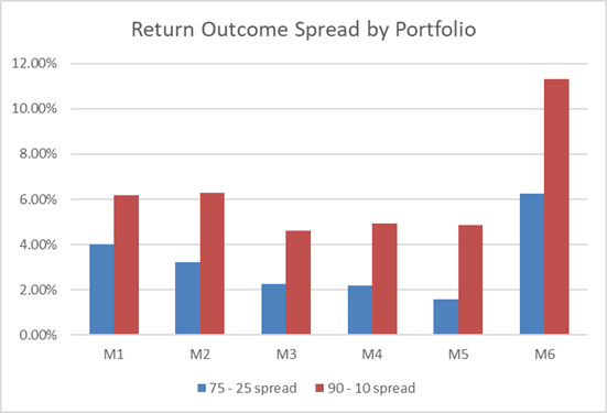
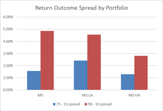
Let us look at these 6 portfolios using our summary charts from above to see the impact of portfolio constraints clearly.
First, we will look at the return spreads by portfolio. We can see the 75th – 25th spread steadily dropped as we added new constraints from M1 through M5 before spiking up with the introduction of the M6 constraint. Note the change from M3 to M4 is relatively minor, while the changes from M1 to M2 or M4 to M5 are relatively larger.
As described above, as the portfolio shape definition became more constrained the spread of possible outcomes gradually tightened.
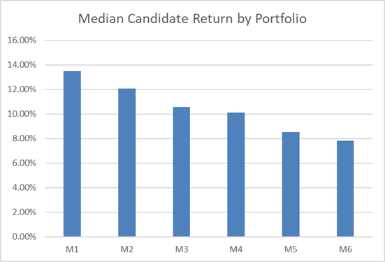
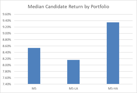
The same dynamic is visible here in median return – additional constraints slowly lowered the median return. All things equal, the PM might expect to generate increasingly lower returns as the portfolio becomes more constrained.
This table summarizes each of the Candidate Portfolio Analysis outputs shown above.
Understanding this Impact is Non-intuitive, but Important
It would be difficult for PMs to have an intuitive understanding of the impact of each of the prior constraints.
When the sector constraint was applied in portfolio M4, the results differed relatively little from portfolio M3. However, when we re-added the constraint that all assets must be included to produce portfolio M5, the results changed much more substantially. Grasping this for each set of constraints placed on a portfolio is difficult without a way to illustrate the impact.
On the other side of the spectrum, the constraint added to generate M6 – that any position must either be a minimum of 3% above benchmark weight or not in the portfolio at all – produced huge changes in possible outcomes. Far fewer compliant candidate portfolios could be made subject to that constraint, leading to much more variable outcomes driven by single stock idiosyncratic risk.
With Constraints Set, Other Decisions Also Navigate Outcomes
The Candidate Portfolio lens can also help PMs think about different objectives within a fully defined set of constraints. Let’s use portfolio M5 above as a “live” example.
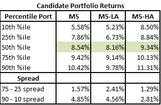
Given this set of possible outcomes, the PM could choose to focus on several different objectives. Examples include relatively higher / lower active share, relatively more / less in the highest conviction ideas, etc. Let us look at active share for our final illustration.
Targeting by Active Share Gives a Subset with the Possible Portfolios
If the PM chooses a portfolio construction with relatively lower active share that places them within a subset of the possible portfolios shown above. Here we look at the bottom quintile of active share portfolios from the Candidate Portfolios above.
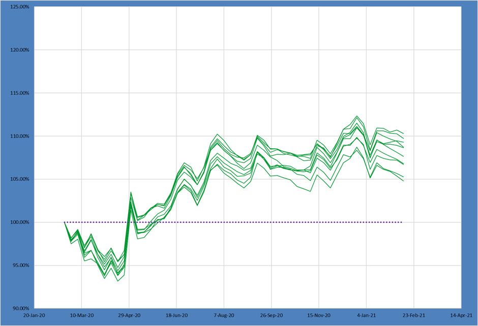
The lower active share portfolios look relatively different from the full set of Candidates. We can see using our median and spread metrics both a lower median outcome and a wider 75th – 25th spread.
This suggests this PM would benefit from taking MORE active share rather than less given this set of alpha ideas and portfolio shape!

For comparison, the following chart shows the top quintile of Candidate Portfolios from our M5 set by active share.
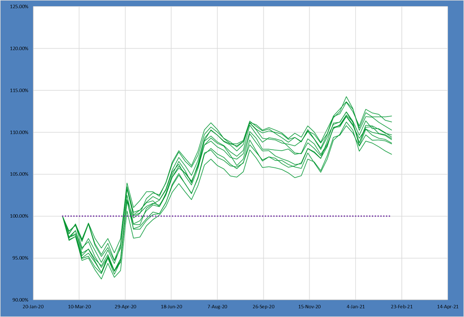
The higher active share portfolios have both a higher median return and a small spread. Given this set of ideas the PM would definitely benefit from pursuing a higher active share expression of their ideas!

We can again summarize this using the methodology we used to describe the different types of constraints above. The takeaway for this PM should be quite clear – taking more active risk with this portfolio could lead to better possible outcomes.
Understanding Impact of Constraints Allows Better Decision-Making
PMs need to understand the impact of portfolio constraints on portfolio outcomes to make more informed portfolio construction decisions.
That may entail mitigating disproportionately impactful hard constraints they cannot change. or modifying soft constraints to produce a set of outcomes they are more comfortable with. Without considering constraints they fly blind without a concrete understanding of the impact of their portfolio shape decisions.
Using a few simple metrics, the Candidate Portfolio Analysis tool can help managers better understand their portfolio shaping decisions.
By thinking critically about each constraint and quantifying its potential impact, PMs can make more better portfolio construction decisions and improve their portfolio outcomes.
To see the potential impact of improved portfolio construction on your portfolio and learn more about refining your team’s portfolio construction process, get in touch with the Sherpa team or sign up for the SFT mailing list here.